Why Quantum Neural Networks Stop Learning: Barren Plateaus and Dynamical Lie Algebras

Quantum neural networks can grow more expressive while becoming almost impossible to train. In deep, sufficiently random parametrized circuits, the typical gradient can shrink exponentially with the number of qubits, leaving a classical optimizer unable to distinguish a useful update from measurement noise. Modern dynamical Lie algebra methods identify when the collapse comes from the circuit itself—and when it comes from the initial state, the measured observable, or the physical noise.

Parameterized quantum circuits are frequently described as neural networks whose adjustable weights happen to be quantum gate angles. That description captures the outer optimization loop, but it leaves out the central difficulty. A classical algorithm proposes new parameters, the quantum circuit runs, and measurements estimate an objective. If almost every randomly sampled parameter vector produces a gradient indistinguishable from zero, the optimization loop has no affordable directional information. The model may have a perfectly good global minimum and enough gates to represent it; neither fact establishes that gradient-based training will find the minimum. [1][2]

There has been a major shift in how theorists analyze this phenomenon. The original barren-plateau results connected trainability to concentration of measure in high-dimensional state spaces. Subsequent work showed that global loss functions can be disastrous even for circuits with no entanglement. Two complementary papers published in 2024 made circuit-generated Lie algebras central to the analysis: one supplied exact loss-variance relations for sufficiently mixed Lie-group circuit ensembles, and the other obtained exact gradient-variance formulas for Lie-algebra-supported observables. A 2026 QAOA study derived explicit algebras for certain graph families and used them to characterize the absence of barren plateaus. [1][2][5][6][9]

The signal that disappears

For an $n$-qubit system with input density matrix $\rho$, parameterized unitary $U(\boldsymbol{\theta})$, and Hermitian cost observable $H$, the expected loss has the form

$E(\boldsymbol{\theta})=\operatorname{Tr}[U(\boldsymbol{\theta})\rho U^\dagger(\boldsymbol{\theta})H],\qquad E(\boldsymbol{\theta})=\langle 0|U^\dagger(\boldsymbol{\theta})HU(\boldsymbol{\theta})|0\rangle\quad(\rho=|0\rangle\langle0|).$

Its derivative with respect to angle $\theta_k$ is an observable quantity estimated from quantum measurements. A barren plateau describes a family of circuits and an initialization distribution for which the variance of that derivative decays exponentially with system size. A conventional criterion is

$\operatorname{Var}_{\boldsymbol{\theta}}[\partial_{\theta_k}E]\in\mathcal{O}(b^{-n}),\qquad b>1.$

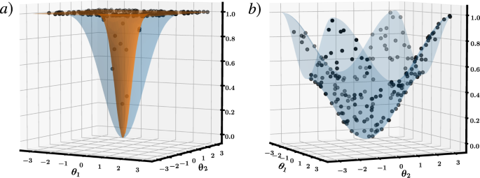
The derivative need not vanish exactly, and a barren plateau need not resemble a smooth valley containing a single narrow minimum. Typically, its mean is zero and its fluctuations about zero become exponentially small. A direct consequence of Chebyshev's inequality is that, when the mean is zero, $\Pr(|\partial_kE|\geq\varepsilon)\leq\operatorname{Var}(\partial_kE)/\varepsilon^2$ for a fixed threshold $\varepsilon>0$. Random initializations overwhelmingly land where ordinary gradient estimates carry almost no information. [1]

In real devices, even a theoretically nonzero derivative is useful only if its sign and magnitude can be measured. Suppose the angle enters as a gate $\exp(-i\theta_kP/2)$, where $P$ is a Pauli string with $P^2=I$. Under the usual parameter-shift assumptions its derivative can be measured by running the same circuit at two shifted angles:

$\partial_{\theta_k}E=\frac{E(\boldsymbol{\theta}+\frac{\pi}{2}\mathbf e_k)-E(\boldsymbol{\theta}-\frac{\pi}{2}\mathbf e_k)}{2}.$

Estimating each expectation with independent measurement shots incurs statistical error that typically falls as $M^{-1/2}$, where $M$ is the shot count. If the signal is of order $b^{-n/2}$ but the single-shot fluctuations remain order one, maintaining fixed signal-to-noise ratio requires $M$ of order $b^n$. This is a conditional estimate, not a universal lower bound on every gradient protocol; it explains why an experimentally finite shot budget can make a formally differentiable model untrainable.

Haar randomness and the limits of expressibility

An $n$-qubit Hilbert space has dimension $d=2^n$. The special unitary group $SU(d)$ has real Lie algebra dimension $d^2-1=4^n-1$. Deep, unstructured circuits with suitable random gates can reproduce statistical properties of Haar-random unitaries. For many cost-variance calculations, complete Haar randomness is unnecessary: an approximate unitary 2-design already matches the relevant second moments closely enough to yield similar concentration. That makes the dangerous regime accessible to circuits of finite depth rather than only to fantastically large generic matrices. [1][3]

Expressibility describes what states or operations an ansatz can represent, whereas trainability concerns whether measurements at its initialized parameters allow efficient progress toward a target. They are not interchangeable. A broadly expressive gate family can induce a narrow distribution of loss values, and restricted gate families can preserve a useful gradient signal. Yet the converse does not follow: simply reducing circuit expressibility cannot guarantee training success. The observable and the prepared state can independently suppress gradients, and hardware noise can do so even in an ideal ansatz that looks favorable. [2][5][7]

An exact barren plateau without entanglement

The most effective counterexample begins with independent single-qubit rotations. Prepare $|0\rangle^{\otimes n}$ and apply a $Y$ rotation on each qubit, with each angle independently uniform on $[0,2\pi)$. Nothing entangles the qubits:

$U(\boldsymbol{\theta})=\bigotimes_{j=1}^{n}\exp(-i\theta_jY_j/2).$

Consider first a global fidelity objective: the probability that a computational-basis measurement returns the all-zero string. The cost is $C_{\mathrm G}=\prod_{j=1}^n\cos^2(\theta_j/2)$. Its derivative is a product over all the other qubits. Averaging over the angles, using $\mathbb E[\sin^2\theta]=1/2$ and $\mathbb E[\cos^4(\theta/2)]=3/8$, gives the exact variance

$\partial_{\theta_k}C_{\mathrm G}=-\tfrac12\sin\theta_k\prod_{j\neq k}\cos^2(\theta_j/2),\qquad\operatorname{Var}(\partial_{\theta_k}C_{\mathrm G})=\tfrac18(\tfrac38)^{n-1}.$

The gradients disappear exponentially even though the ansatz has no entangling gates. Instead measure the average local failure probability, $C_{\mathrm L}=1-\frac1n\sum_{j=1}^n\cos^2(\theta_j/2)$. Its derivative variance is radically different:

$\partial_{\theta_k}C_{\mathrm L}=\frac{\sin\theta_k}{2n},\qquad\operatorname{Var}(\partial_{\theta_k}C_{\mathrm L})=\frac{1}{8n^2}.$

Both costs are minimized at the all-zero target state in this product-state example. Nevertheless, a global objective gives exponential concentration and the local objective only polynomial concentration. Cerezo and collaborators analyzed this example and generalized the lesson to certain shallow alternating-layer architectures, proving that local costs can avoid exponential decay for appropriate depths and assumptions. A local replacement objective for a different task must still be justified: making a loss trainable is useless if minimizing it no longer solves the original problem. [2]

Constructing a dynamical Lie algebra from the gates

The dynamical Lie algebra, or DLA, is the real Lie algebra generated by the skew-Hermitian gate generators and all their nested commutators. For a collection of Hermitian operators $H_1,\ldots,H_K$, write

$\mathfrak g=\operatorname{Lie}_{\mathbb R}\langle iH_1,\ldots,iH_K\rangle,\qquad[A,B]=AB-BA.$

The commutator is the crucial operation. If a circuit can rotate a single qubit about $X$ and $Z$, those generators produce a rotation direction about $Y$ through the Pauli commutation relations. Together, the three independent directions give $\mathfrak{su}(2)$. Repeating a full one-qubit algebra independently on $n$ qubits yields a direct sum $\mathfrak{su}(2)^{\oplus n}$ of dimension $3n$. With suitable entangling couplings and no protecting symmetries, the closure can expand all the way to $\mathfrak{su}(2^n)$, whose dimension is $4^n-1$.

For the product-$Y$ circuit just analyzed, all $iY_j$ commute, so its DLA is an abelian algebra of dimension $n$. The global fidelity still has an exponentially small gradient variance. This is the precise reason the statement “polynomial DLA dimension prevents barren plateaus” cannot stand as a general theorem. A restricted algebra blocks one possible concentration mechanism, but says nothing by itself about how a chosen observable samples the accessible directions. [4][5]

Algebraic purity and the 2024 concentration theorem

Ragone and collaborators formalized the relationship by projecting the initial state and measured observable onto the vector space of Hermitian generators associated with $\mathfrak g$. Let $\{B_a\}$ be a Hilbert–Schmidt orthonormal basis for $i\mathfrak g$. Define the squared norm of the projected operator by

$\mathcal P_{\mathfrak g}(A)=\sum_{a=1}^{\dim\mathfrak g}\left|\operatorname{Tr}(B_a A)\right|^2.$

This algebraic purity is distinct from the usual state purity $\operatorname{Tr}(\rho^2)$. It measures the overlap with a distinguished set of observables generated by the circuit. A conventionally pure state can have little accessible algebraic signal, and a measurement that is global across the qubits may overlap poorly with this algebra. The measure also connects to generalized entanglement, defined relative to accessible observables rather than a preferred spatial partition into qubits. [5]

For a simple DLA, a sufficiently deep circuit whose ensemble mixes according to the required second moments, and under the theorem's support assumptions on the state or observable, the variance of the loss obeys

$\operatorname{Var}_{U\sim G}[\operatorname{Tr}(U\rho U^\dagger O)]=\frac{\mathcal P_{\mathfrak g}(\rho)\mathcal P_{\mathfrak g}(O)}{\dim\mathfrak g}.$

For a semisimple DLA the expression becomes a sum over its simple ideals, with central contributions handled separately. The formula explains how three effects can reduce a trainable signal: a very large dynamical algebra, a small algebraic projection of the state, or a small algebraic projection of the measured operator. In other words, avoiding Haar-like expressibility is insufficient if state preparation or measurement still suppresses information. The result also supplies a framework for understanding certain noise-induced effects. [5]

An important distinction is often lost when citing these results. Ragone and collaborators establish an exact relation for cost-function variance, from which additional trainability bounds follow. Fontana and collaborators develop exact formulas for gradient variance using the adjoint representation when the observable is Lie-algebra-supported and the specified mixing conditions apply. Their papers are complementary, but the loss-variance equation above should not be silently presented as an identity for every parameter derivative. [5][6]

Why a polynomial-sized algebra can still fail

If $\dim\mathfrak g$ increases only polynomially with $n$, the denominator in the single-simple-algebra formula does not, by itself, enforce exponential concentration. The state and observable projections can still decrease exponentially, however, and the exact formula does not automatically apply when a circuit is too shallow to sample the corresponding group appropriately. The product-$Y$ counterexample also has a global measurement outside the tiny generator algebra, exposing the limitation directly.

A small algebra creates a second problem: it may make the circuit insufficiently expressive for the target. Restricting evolution to a conserved particle-number sector is sensible when the physics preserves particle number; it is dangerous when the training labels require transformations that cross those sectors. Algebraic structure is useful only when it is chosen with the state, task, and measurement in mind. A model with large gradients but the wrong reachable states is still a poor model.

Symmetry-preserving compound circuits

Fontana and collaborators examined quantum compound ansätze built from structured rotations, including fermionic beam-splitter gates. Their effective groups are representations of $SO(n)$ or $SU(n)$ acting on exponentially large qubit registers, but the corresponding Lie algebras grow only polynomially with the register size. Such circuits preserve Hamming weight, so the state space decomposes into sectors that can be studied separately. The adjoint representation allows the gradients of Lie-algebra-supported observables to be analyzed directly. [6]

For specified computational-basis initial states, the paper established polynomial lower bounds, including $\Omega(n^{-3})$, on gradient variance in the supported setting. For the uniform superposition state $|+\rangle^{\otimes n}$, the relevant scaling is $\Theta(n^{-2})$. The authors compared exact predictions against numerical estimates at multiple system sizes. Those demonstrations are meaningful precisely because the assumptions are explicit: a restricted gate family, an identified Lie group, prescribed initial states, a supported measurement, and a controlled parameter distribution. [6]

These compounds do not prove the practical superiority of quantum neural networks over classical models. They supply architecture families in which a particular source of trainability failure can be mathematically ruled out. Whether a specific classifier generalizes, whether an optimizer finds a useful target, and whether implementation noise erases the advantage remain separate empirical questions.

A 2026 example: QAOA on cycle graphs

Graph-structured quantum approximate optimization algorithms offer another test of algebraic reasoning. In QAOA, the cost Hamiltonian encodes the graph optimization objective and a mixing Hamiltonian generates transitions among basis states. Their alternating exponentials generate a DLA whose closure can reflect the graph itself. Jonathan Allcock, Miklos Santha, Pei Yuan, and Shengyu Zhang derived analytical results for MaxCut-type QAOA families, including cycles and complete graphs, in a paper published in Quantum in May 2026. [9]

For an $n$-vertex cycle, their DLA decomposes into a two-dimensional center and a semisimple component isomorphic to $n-1$ copies of $\mathfrak{su}(2)$, a total dimension of $3n-1$. They obtained an exact cost-variance expression and proved the absence of barren plateaus in the construction studied. For complete graphs, they bounded the algebra dimension by $\mathcal O(n^3)$ and produced an explicit basis. The results show how graph topology can be converted into an algebraic statement about circuit statistics. They do not imply that every QAOA instance is efficiently solvable: landscapes without barren plateaus may still contain difficult local optima, expensive measurement requirements, and other computational bottlenecks. [9]

A practical audit before the first training run

For a proposed variational quantum model, the first step is to list every independent parameter generator and compute its commutator closure for increasing system sizes. On small registers, Pauli-string representations and exact symbolic linear algebra can provide the DLA dimension; numerical rank tests require suitable tolerances and verification. Identify all operators commuting with the generated algebra, because conserved quantities decompose the representation into invariant sectors. A circuit that is universal within one sector may be unable to reach a target lying outside that sector. [4][6]

The second step is to examine the actual data-encoding state and cost observable. Does the measurement belong to the dynamical algebra? Is the input strongly aligned with the accessible Lie-algebra directions? Can the loss be localized without changing its solution set? Estimate the variance of gradients over the initialization distribution across several register sizes, and record the confidence intervals and shot budgets. Only then should one fit an exponential or polynomial scaling law. The choice of scaling variable and the distribution of random parameters are part of the scientific result, not a plotting afterthought.

Third, test circuit depth and noise separately. A deep randomized ansatz may approach the mixing assumptions of a Lie-group theorem; a shallow ansatz may not. Noise can also contract the measured signal even for ideal circuits whose algebra is favorable. Compare meaningful loss values as well as gradient sizes, and include a classical baseline when the model claims an advantage on a learning or optimization task. A theoretically favorable gradient distribution is a prerequisite for certain optimizers, not a complete measure of utility. [7][8]

The engineering meaning of trainability

Quantum computing hardware makes the stakes of these mathematical distinctions concrete. Gate errors, calibration drift, finite shot counts, readout errors and compilation constraints are all paid for in laboratory time and physical resources. An ansatz whose theoretical gradients require exponentially many shots cannot simply be rescued by saying that its optimizer is more sophisticated. Conversely, a symmetry-matched gate family may need fewer exploratory experiments because its reachable directions have been understood in advance. The relationship between gate architecture and trainability therefore has direct implications for useful hardware budgets.

The deeper methodological change is to stop treating variational circuits as arbitrary sequences of trainable quantum gates. Their generators define a Lie algebra. That algebra interacts with the input state and observable, and the interaction helps determine the statistics available to the learning algorithm. The practical design task is to select transformations with enough freedom to represent the target while preserving enough structure for gradients to remain measurable. The 2024 results turn that principle into equations; the 2026 QAOA analysis shows that in some algorithm families it can be calculated almost graph by graph.

References

[1] McClean, J. R. et al., Barren plateaus in quantum neural network training landscapes, Nature Communications 9, 4812 (2018). Original paper.

[2] Cerezo, M. et al., Cost function dependent barren plateaus in shallow parametrized quantum circuits, Nature Communications 12, 1791 (2021). Original paper.

[3] Holmes, Z. et al., Connecting Ansatz Expressibility to Gradient Magnitudes and Barren Plateaus, PRX Quantum 3, 010313 (2022). Original paper.

[4] Larocca, M. et al., Diagnosing Barren Plateaus with Tools from Quantum Optimal Control, Quantum 6, 824 (2022). Original paper.

[5] Ragone, M. et al., A Lie algebraic theory of barren plateaus for deep parameterized quantum circuits, Nature Communications 15, 7172 (2024). Original paper.

[6] Fontana, E. et al., Characterizing barren plateaus in quantum ansätze with the adjoint representation, Nature Communications 15, 7171 (2024). Original paper.

[7] Wang, S. et al., Noise-Induced Barren Plateaus in Variational Quantum Algorithms, Nature Communications 12, 6961 (2021). Original paper.

[8] Larocca, M. et al., Barren plateaus in variational quantum computing, Nature Reviews Physics 7, 174–189 (2025). Review.

[9] Allcock, J., Santha, M., Yuan, P. and Zhang, S., On the dynamical Lie algebras of quantum approximate optimization algorithms, Quantum 10, 2119 (2026). Original paper.

Cover photograph: Google Sycamore superconducting quantum processor on display at the Deutsches Museum, Munich. Photograph by Coldupnorth, Wikimedia Commons, CC BY-SA 4.0.