Six Seconds of Gamma Rays: How Bayesian Physics Locates Invisible Sources

What six seconds of radiation can reveal

A helicopter passes over a field at roughly ten metres per second. A scintillation detector aboard the aircraft records a sequence of gamma-ray spectra, each lasting only one second. Somewhere beneath the flight path are radioactive sources whose positions and strengths are unknown. The spectra are mixtures: natural potassium, uranium and thorium contribute photons, atmospheric radon contributes additional background, and the aircraft itself changes the radiation reaching the detector. Identifying a single spectral line is not enough to reconstruct the scene. The question is whether six brief observations can jointly determine which radionuclides are present, where they lie and how much activity they contain.

In research published on 26 October 2026, David Breitenmoser, Alberto Stabilini, Malgorzata Magdalena Kasprzak and Sabine Mayer answered that question experimentally using high-fidelity radiation transport and Bayesian inference [1]. Their airborne measurements recovered the correct source mixture with strong model-comparison evidence, localized sources to within two metres and estimated their activities within a few percent of independent laboratory values. The measurements were collected during a 2022 Swiss field exercise; the 2026 advance lies in the quantitative inversion of these data. A detector moving through an uncertain radiation field can now be interpreted as a physical measurement system rather than a simple counter of peaks.

The study illustrates a general principle in experimental physics. When data are sparse, progress can come from making the forward model more faithful and the uncertainty model more honest. The same logic connects nuclear detection with astronomy, geophysics, medical imaging and other inverse problems in which a small number of observations must constrain a hidden physical distribution.

A spectrum is a record of interactions, not a list of isotopes

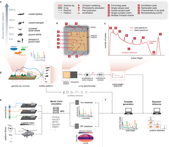
A gamma-ray photon can undergo photoelectric absorption, Compton scattering or, at sufficiently high energy, pair production. A scintillator records the light produced by energy deposited in its material, so the measured pulse height need not equal the energy of the incoming photon. A monoenergetic source produces a full-energy peak together with a Compton continuum, escape features and secondary structures. Atmospheric attenuation, ground backscatter and shielding by the aircraft modify those features before the photons reach the detector [1,2].

The Swiss Airborne Gamma-Ray Spectrometry system uses approximately 17,000 cubic centimetres of thallium-doped sodium iodide, NaI(Tl), carried aboard an AS332M1 Super Puma helicopter. Four scintillation crystals are combined into a response with 1,008 channels covering roughly 50 keV to 3 MeV. The instrument samples at 1 Hz during the field experiments. Its large crystal volume helps collect photons, but the modest energy resolution of NaI(Tl) means that closely spaced contributions are often not cleanly separable by eye [1].

The detector response can be written as a linear operator acting on an incoming photon flux. If $\Phi(E,\Omega,t)$ is the differential flux as a function of energy, direction and time, and $R_j(E,\Omega;\mathbf d_t)$ is the probability-weighted response in pulse-height channel $j$ for platform state $\mathbf d_t$ , then the expected count rate is schematically

\lambda_j(t)=\int R_j(E,\Omega;\mathbf d_t)\Phi(E,\Omega,t)\,\mathrm dE\,\mathrm d\Omega+b_j(t).

Here $b_j$ represents backgrounds not already included in the flux term. The essential point is that every channel receives contributions from many incident energies and directions. Inverting the spectrum requires a model of the entire interaction chain, not merely a table of isotope emission energies.

**Figure 1.** The forward chain from source emission and gamma-ray transport to detector pulse heights, precomputed response libraries and Bayesian inference. The original schematic compares mobile platforms and identifies physical processes that shape a measured spectrum. Source: D. Breitenmoser et al., Nature Communications 17, 10913 (2026), Fig. 1, reproduced unmodified under CC BY 4.0.

Building a forward model that moves with the helicopter

The new framework separates the expensive particle-transport calculation from the repeated evaluations needed for statistical inference. Detailed radiation-transport simulations first generate instrument response functions and gamma-ray flux libraries for the source, environment and aircraft geometry. At inference time, these precomputed components are assembled into a predicted spectrum for each candidate source position, activity and measured platform state. This retains the scattering and shielding effects of a realistic moving platform without rerunning a full Monte Carlo calculation for every possible parameter value [1,2].

Let $\xi_s$ denote the activity or activity concentration of source component $s$ , and let $\psi_{j,s}(\mathbf x_s,\mathbf d_t)$ be its predicted count-rate template in channel $j$ for source position $\mathbf x_s$ and platform state $\mathbf d_t$ . A useful discretized forward model is

\mu_{tj}=\Delta t_t\left[\sum_{s=1}^{N_s}\xi_s\psi_{j,s}(\mathbf x_s,\mathbf d_t)+b_{tj}\right].

The expected count $\mu_{tj}$ is the quantity against which the observed integer count $y_{tj}$ is compared. The model remains linear in the source strengths when locations and conditions are fixed, but it is nonlinear in source location because changing the geometry alters attenuation, scattering and solid angle. The full analysis also carries nuisance parameters describing effects that are not known perfectly.

This factorization matters computationally. Earlier work by the same team demonstrated a roughly seven-order-of-magnitude acceleration of full-spectrum template evaluation while preserving close agreement with brute-force radiation transport [2]. The 2026 inference study exploits that acceleration to perform many thousands of forward-model evaluations within a practical analysis. The gain comes from amortizing a costly physical calculation across many candidate interpretations of the data; it is not a claim that Monte Carlo radiation transport itself has become seven orders of magnitude faster.

Why ordinary Poisson counting is not always enough

Ideal radioactive decays lead naturally to a Poisson count model: if the expected number of events in a channel is $\mu$ , the probability of observing $y$ counts is $P(y\mid\mu)=e^{-\mu}\mu^y/y!$ . The Poisson model fixes the variance equal to the mean. A moving detector, however, can encounter fluctuating backgrounds, detector pileup, imperfectly represented geometry and residual calibration mismatch. These effects can make the observed variation larger than the ideal model predicts.

Breitenmoser and colleagues use a negative-binomial likelihood with an inferred dispersion parameter $\alpha$ . One convenient parameterization has

\operatorname{E}[Y]=\mu,\qquad \operatorname{Var}(Y)=\mu+\alpha\mu^2,\qquad \alpha\geq0.

In the limit $\alpha\to0$ , the distribution approaches Poisson counting. Positive $\alpha$ permits extra variability while retaining the discreteness of observed counts. This flexibility prevents a slightly inaccurate forward model from automatically producing unrealistically narrow uncertainty intervals. It also means that an inferred nonzero dispersion parameter cannot, by itself, identify the physical cause of the excess variation [1].

For a set of spectra, the likelihood is a product over measurement times and spectral channels, conditioned on the predicted means and dispersion. In practice the logarithm of this likelihood is evaluated to avoid numerical underflow. Because the analysis uses the entire spectrum, weak information distributed across many channels can contribute to distinguishing two competing source hypotheses, even when their most conspicuous peaks overlap.

**Figure 2.** Measured and posterior-predicted pulse-height spectra for stationary hover flights above separate caesium-137 and barium-133 sources, compared across one-second, five-second and approximately five-minute acquisitions. Source: D. Breitenmoser et al., Nature Communications 17, 10913 (2026), Fig. 2, reproduced unmodified under CC BY 4.0. Helicopter line art within the original figure was adapted by the authors from Jetijones, CC BY 3.0.

Bayesian inference turns spectral ambiguity into probabilities

The unknown parameter vector $\boldsymbol\theta$ contains source strengths, source positions and nuisance parameters. For a specified source-mixture hypothesis $S$ , Bayes' theorem gives

p(\boldsymbol\theta\mid D,S)=\frac{p(D\mid\boldsymbol\theta,S)\,p(\boldsymbol\theta\mid S)}{p(D\mid S)}.

The prior $p(\boldsymbol\theta\mid S)$ describes the admissible parameter space, the likelihood scores agreement with the observed spectra $D$ , and the posterior combines both. The denominator is the evidence $Z_S=p(D\mid S)$ , obtained by integrating likelihood times prior over the model parameters. Unlike a best-fit score alone, the evidence accounts for how much of a model's allowed parameter space predicts the data well.

For two candidate mixtures, the Bayes factor $B_{12}=Z_{S_1}/Z_{S_2}$ compares their support under the chosen priors. The investigators explicitly compare background-only, single-source and dual-source hypotheses rather than assuming in advance which anthropogenic isotopes are present. They sample parameter posteriors with an affine-invariant ensemble Markov-chain Monte Carlo method and estimate evidences for the competing models [1,8].

The distinction between a posterior credible interval and a frequentist confidence interval is important here. A credible interval reports a probability statement conditional on the data, the chosen likelihood and the prior assumptions. Its numerical width is meaningful only to the extent that the physical response model and the error model are adequate. Posterior predictive checks, in which simulated spectra from the fitted model are compared with actual observations, therefore provide an essential second test beyond reporting a narrow parameter interval.

**Figure 3.** Joint posterior distributions for anthropogenic source activities, natural radionuclide concentrations, atmospheric radon adjustment and negative-binomial dispersion. Diagonal panels show marginal distributions; off-diagonal panels show parameter correlations and credible contours. Source: D. Breitenmoser et al., Nature Communications 17, 10913 (2026), Fig. 3, reproduced unmodified under CC BY 4.0.

The controlled benchmark: one second, five seconds and five minutes

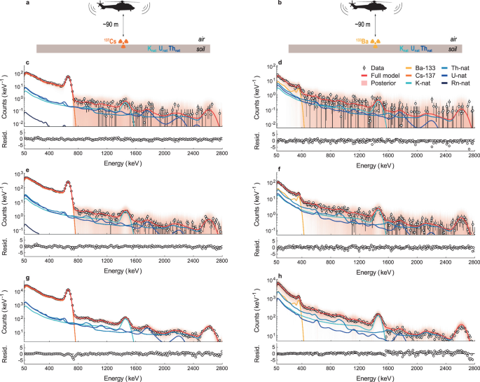
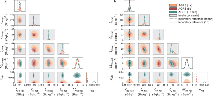
The experimental data were collected on 16 June 2022 at the Thun training ground in Switzerland. In the controlled configuration, the helicopter hovered approximately 90 metres above a sealed source for about five minutes. The source locations were known, allowing the inference to concentrate on source activity and natural background contributions. The team analyzed one-second and five-second subsets as well as the full acquisition, comparing inferred activities with independent laboratory assay values [1].

The sources were caesium-137 and barium-133, two nuclides with different gamma-emission patterns. The model also included natural potassium, thorium and uranium contributions and a variable atmospheric-radon term. Background flights over nearby Lake Thun helped constrain intrinsic, cosmic and atmospheric contributions. Ground measurements at 23 locations provided independent constraints on the natural radioactivity of the site. These separate measurements matter because a Bayesian model cannot validate itself simply by returning a plausible-looking posterior.

Across the hover tests, the posterior median activities of the anthropogenic sources differed from the laboratory references by less than two percent and remained consistent within combined one-standard-deviation uncertainties [1]. The natural radionuclide estimates agreed more broadly with field reference ranges, where spatial heterogeneity and higher-energy counting noise create larger uncertainty. The result demonstrates that full-spectrum inference can use short acquisitions without treating the entire natural background as a single featureless offset.

The moving benchmark: six one-second spectra

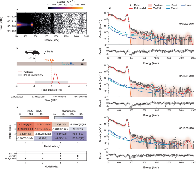
The more demanding experiments flew over the sources at about 30 metres above ground and approximately 10 metres per second. The investigators analyzed six consecutive one-second spectra centered on the peak count-rate region. During those six seconds, source–detector distance and orientation changed, and so did the natural background contribution along the path. The model treated the source location as unknown, allowed natural activity concentrations to vary between spectra and compared all candidate mixtures of caesium-137 and barium-133 [1].

For the barium-only case, the recovered activity was $0.473^{+0.012}_{-0.012}\,\mathrm{GBq}$ . The estimated source location was within two metres of the reference position, and the correct isotope hypothesis was decisively preferred over the alternatives. This is a demanding identification problem because barium-133 emits several gamma lines in a lower-energy region where attenuation, detector response and natural backgrounds complicate interpretation.

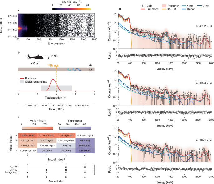
**Figure 4.** Single-pass barium-133 experiment: time-resolved spectra, spatial source posterior, model-evidence comparisons and fitted spectral components. The inference uses six one-second observations rather than a long stationary exposure. Source: D. Breitenmoser et al., Nature Communications 17, 10913 (2026), Fig. 4, reproduced unmodified under CC BY 4.0. Helicopter line art within the original figure was adapted by the authors from Jetijones, CC BY 3.0.

For the caesium-only case, the inferred activity was $8.88^{+0.14}_{-0.12}\,\mathrm{GBq}$ , again within two percent of the independently calibrated value. Caesium-137 has a prominent 662-keV gamma signature, but that recognizable line does not eliminate the need to model the continuum, aircraft shielding, backgrounds and changing source geometry. The data also show residual distortions at higher energies near the maximum count rate, indicating that even an accurate overall reconstruction can leave localized response-model discrepancies.

**Figure 5.** Single-pass caesium-137 experiment: count-rate evolution, spatial localization, competing isotope models and posterior predictive spectra. Residual spectral distortions remain visible in parts of the high-count-rate response. Source: D. Breitenmoser et al., Nature Communications 17, 10913 (2026), Fig. 5, reproduced unmodified under CC BY 4.0. Helicopter line art within the original figure was adapted by the authors from Jetijones, CC BY 3.0.

Two sources beneath the same flight path

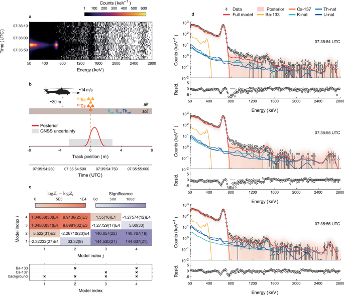
The most revealing test placed the two anthropogenic sources less than 20 centimetres apart. Their physical separation was far below the spatial resolution available to the airborne system, so the inference was effectively tasked with recovering two source strengths at a common location. The much stronger caesium contribution partially masked the barium signature. Nevertheless, the model comparison preferred the two-source hypothesis, and the inferred activities were $0.49^{+0.14}_{-0.16}\,\mathrm{GBq}$ for barium-133 and $8.92^{+0.23}_{-0.21}\,\mathrm{GBq}$ for caesium-137 [1].

The barium interval in this mixed case is noticeably wider than in the barium-only case. That widening is physically appropriate: the data provide less independent information about a weak source when its signal is superposed on a stronger source and variable background. The point estimates remain within four percent of their laboratory references, but the uncertainty is not uniformly at the percent level. Distinguishing point-estimate accuracy from posterior precision is essential to interpreting the result.

The paper reports log Bayes factors exceeding 15 against the best competing model in all three single-pass scenarios, corresponding under the authors' stated conservative calibration to more than five Gaussian-equivalent standard deviations [1]. That conversion is a reporting convention tied to model comparison and its assumptions, not a universal identity between Bayesian evidence and a frequentist detection significance. The direct result is that the correct source mixture received much greater integrated likelihood support under the candidate models and priors examined.

**Figure 6.** Co-located barium-133 and caesium-137 sources: the dual-source flight spectra, spatial posterior, model-comparison evidence and decomposition of the overlapping radiation signatures. Source: D. Breitenmoser et al., Nature Communications 17, 10913 (2026), Fig. 6, reproduced unmodified under CC BY 4.0. Helicopter line art within the original figure was adapted by the authors from Jetijones, CC BY 3.0.

The physical meaning of an inferred location

A source is not localized because a detector sees a narrow image of it. A conventional NaI(Tl) spectrometer measures energies, not incoming photon directions. Location information arises indirectly because the count rate and spectral shape change as the aircraft moves. The flight path supplies multiple geometrical views of the same radiation field, and the forward model predicts the response from each hypothetical source position. A spatial posterior emerges from the joint consistency of those predictions with the time series.

This is closely related to inverse imaging problems in which multiple projections constrain an otherwise hidden distribution. Free-moving gamma-ray imaging has previously combined radiation measurements with scene geometry and motion tracking to reconstruct activity in three-dimensional environments [3]. The Swiss experiment differs in its emphasis on full-spectrum isotope-mixture identification and calibrated activity inference using a detailed aircraft response. Both approaches show that motion can be a source of information rather than only a nuisance to correct.

There is a geometric floor to what such data can establish. The study's sub-two-metre source-location accuracy is comparable to the positioning uncertainty of the aircraft's onboard navigation system [1]. It should not be read as evidence that a non-imaging detector has achieved centimetre-scale spatial resolution, or that two sources separated by 20 centimetres were spatially resolved. In the dual-source case the chemical identities were separated statistically, while their locations were treated as essentially co-located.

From nuclear transport to planetary exploration

Gamma-ray spectroscopy is also a planetary science technique. Galactic cosmic rays interact with planetary regolith, generating secondary particles and gamma rays whose characteristic energies constrain elemental composition. NASA's Mars Odyssey Gamma Ray Spectrometer mapped elemental signatures including potassium, thorium, iron and chlorine; its associated neutron instruments provided information about hydrogen and subsurface ice [9,10]. The Dawn mission used nuclear spectroscopy to constrain hydrogen and other elements in Ceres' regolith, finding evidence consistent with widespread near-surface water ice at mid-to-high latitudes [7].

The connection to the airborne work is methodological rather than a claim of an immediate flight-ready planetary algorithm. Spacecraft encounter different backgrounds, orbital geometries, regolith transport physics and instrument response functions. The new framework's separation of a high-fidelity transport library from statistical inversion could, in principle, support improved uncertainty propagation in orbital mapping. Applying it to a planetary mission would require new calibrated response models, appropriate spatial source parameterizations and validation against independent data.

One especially promising extension is to treat composition as a continuous field rather than a collection of isolated point sources. The forward model would then connect each spectrum to a spatial distribution of elemental or radionuclide abundances, and the posterior would express both the inferred map and the correlations between neighboring regions. Such a problem is computationally larger and more underdetermined than the Thun experiments, but the same probabilistic architecture provides a coherent starting point.

What the experiment has not yet solved

The current demonstrations use a known aircraft and well-characterized field conditions. They do not establish universal accuracy for arbitrary environments, unknown shielding, complex urban structures or distributed contamination. In particular, the measured platform position, orientation and other state variables enter the response templates as known inputs. Their uncertainty is not yet fully propagated through the Bayesian inversion. If navigation errors or unmodeled obstacles alter the response, the resulting credible intervals may understate the true uncertainty [1].

The negative-binomial dispersion parameter helps account for departures from ideal Poisson counts, but it cannot distinguish intrinsic source fluctuations from residual forward-model error, pileup or rapidly varying background. In the moving tests, inferred dispersion is larger than in short hover acquisitions, and the caesium-rich measurements show discrepancies in approximately the 800–1300-keV region. Those observations motivate more detailed treatment of high-count-rate detector behavior and dynamic backgrounds. A flexible likelihood can absorb some mismatch; it does not remove the need to understand its cause.

Computational scaling is another constraint. The study reports complete Markov-chain analyses taking on the order of hundreds of seconds on a single CPU core after response libraries are available [1]. This is practical for post-processing but not yet proof of real-time inference across a large, spatially continuous field with many candidate isotopes. More complex scenes will demand efficient parameterizations, surrogate validation and careful checks that posterior sampling has converged.

Why the result matters

The central achievement is a quantitative agreement between an explicit radiation-transport model, a statistical description of sparse counts and independent physical reference measurements. Six seconds of data were sufficient in the tested scenarios because the model used the information distributed across the entire spectrum and the changing measurement geometry. The inferred isotope mixtures, activities and locations were evaluated together rather than through disconnected peak searches and position estimates.

That synthesis suggests a productive direction for measurement science. Better detectors remain valuable, but an equally important frontier is making more of the information already present in noisy observations. A gamma-ray spectrum is the end of a long chain of physical interactions. Reconstructing that chain probabilistically can turn a fleeting signal into a constrained account of an otherwise invisible source.

References

D. Breitenmoser, A. Stabilini, M. M. Kasprzak and S. Mayer, “Quantitative mobile gamma-ray spectrometry through Bayesian inference,” Nature Communications 17, 10913 (2026), published 26 October 2026. doi:10.1038/s41467-026-78464-2.
D. Breitenmoser, A. Stabilini, M. M. Kasprzak and S. Mayer, “Full-spectrum modeling of mobile gamma-ray spectrometry systems in scattering media,” Physical Review Applied 25, 014044 (2026). doi:10.1103/yhz2-xmby.
D. Hellfeld, M. S. Bandstra, J. R. Vavrek et al., “Free-moving Quantitative Gamma-ray Imaging,” Scientific Reports 11, 20515 (2021). doi:10.1038/s41598-021-99588-z.
M. Salathe et al., “Determining urban material activities with a vehicle-based multi-sensor system,” Physical Review Research 3, 023070 (2021). doi:10.1103/PhysRevResearch.3.023070.
J. C. Curtis et al., “Simulation and validation of the Mobile Urban Radiation Search (MURS) gamma-ray detector response,” Nuclear Instruments and Methods in Physics Research A 954, 161128 (2020). Journal DOI.
S. Agostinelli et al., “GEANT4—a simulation toolkit,” Nuclear Instruments and Methods in Physics Research A 506, 250–303 (2003). doi:10.1016/S0168-9002(03)01368-8.
T. H. Prettyman, N. Yamashita, M. J. Toplis et al., “Extensive water ice within Ceres' aqueously altered regolith: Evidence from nuclear spectroscopy,” Science 355, 55–59 (2017). doi:10.1126/science.aah6765.
J. Goodman and J. Weare, “Ensemble samplers with affine invariance,” Communications in Applied Mathematics and Computational Science 5, 65–80 (2010). doi:10.2140/camcos.2010.5.65.
B. C. Hahn et al., “Mars Odyssey Gamma Ray Spectrometer elemental abundances and apparent relative surface age: Implications for Martian crustal evolution,” Journal of Geophysical Research: Planets 112 (2007). doi:10.1029/2006JE002821.
NASA, “Mars Odyssey Science Instruments: Gamma Ray Spectrometer,” mission instrument documentation. NASA Science.

Cover photograph: U.S. Geological Survey, “The Gamma Ray Spectrometer (GRS),” public-domain image of the Mars Odyssey instrument. Source. The spacecraft instrument illustrates planetary gamma-ray spectroscopy and is distinct from the airborne system used in the 2026 study.