The Wavefunction Detective: How Neural Networks Reconstruct Quantum States

Imagine repeating the same quantum experiment thousands of times. Each time, the apparatus reports only a string of classical outcomes: zero or one, spin up or spin down, perhaps a pattern of bright and dark atoms. Yet the system that generated those outcomes can occupy a wavefunction whose description contains exponentially many complex amplitudes. How can a scientist infer the hidden quantum state from such fragmentary evidence? One answer is to train a neural network to become a statistical detective.

Quantum state tomography is the inverse problem of quantum measurement. We know the preparation and the measurement settings imperfectly, collect repeated outcomes, and attempt to reconstruct the state that explains their statistics. Traditional methods formulate the task as estimating a physical density matrix. Neural approaches instead put a structured probability distribution, a wavefunction or a density operator inside a trainable model. The network's parameters are adjusted until predictions agree with observed frequencies. The important claim is not that a computer can look behind a measurement and discover information unavailable in principle. It is that a learned representation can exploit structure that brute-force reconstruction ignores. [2][4][5]

This question became experimentally concrete when neural reconstruction was applied to Rydberg atom arrays, photonic systems and nuclear magnetic resonance devices. More recent work connects neural models to generalized measurements and classical-shadow protocols. The field is now mature enough to ask a harder question than whether AI can represent a wavefunction: what is actually learned, when is the reconstruction identifiable, and how should success be certified independently of the same data used for training? [5][6][7][8][10]

The information hidden by a single measurement

Consider one qubit. Its pure state can be written in a computational basis using two complex amplitudes constrained by normalization and an irrelevant global phase. Those degrees of freedom reduce to a point on the Bloch sphere, described by two real coordinates. A measurement of the Z observable, however, yields only two possible outcomes and determines just one component of the Bloch vector. The other components remain undetermined. Repeated Z measurements, no matter how precise, cannot tell whether the phase between |0⟩ and |1⟩ is positive, negative or something in between.

|\psi\rangle=\cos\frac{\theta}{2}|0\rangle+e^{i\phi}\sin\frac{\theta}{2}|1\rangle

The probabilities of those two Z outcomes are cos²(θ/2) and sin²(θ/2). They contain no dependence on φ. To infer the azimuthal phase, one needs measurements sensitive to X and Y components, or justified prior restrictions that relate phase to other known properties. This identifiability issue becomes more severe as the number of qubits grows. A neural network cannot conjure an unknown relative phase from observations that provably do not depend on it.

p(0|Z)=\cos^2\frac{\theta}{2},\qquad p(1|Z)=\sin^2\frac{\theta}{2}

For n qubits, a pure state requires amplitudes for 2ⁿ basis strings; accounting for normalization and global phase leaves 2ⁿ⁺¹−2 real parameters. A generic mixed density matrix is even larger: a 2ⁿ × 2ⁿ Hermitian trace-one matrix has 4ⁿ−1 real parameters before enforcing positive semidefiniteness. This is the origin of the exponential difficulty of arbitrary full quantum-state reconstruction, both in measurement resources and in classical processing.

|\psi\rangle=\sum_{z\in\{0,1\}^{n}}\psi(z)|z\rangle,\qquad \rho=\sum_{z,z'}\rho_{zz'}|z\rangle\langle z'|

Those counts are dimensions of generic state families, not universal sample-complexity estimates for every special state. If a system is known to be the unique ground state of a particular local Hamiltonian, a low-entanglement state, or the output of a short known circuit family, the unknowns may admit a much smaller description. Efficient learning is then possible only to the degree those assumptions actually characterize the prepared state. [11][13]

Learning a wavefunction as a probability distribution

A productive mathematical starting point is Born's rule. A measurement in an orthonormal basis yields outcome z with probability |ψ(z)|². If a neural model represents this probability, maximum likelihood can fit it to the observed outcome frequencies without enumerating every possible string in a large table. The trained model can generate new synthetic measurement outcomes, estimate correlations, and, with suitable assumptions, furnish a compact representation of the underlying state.

p_{\theta}(z)=\frac{|\psi_{\theta}(z)|^2}{\sum_{z'}|\psi_{\theta}(z')|^2},\qquad \mathcal L(\theta)=-\sum_{z\in\mathcal D}\log p_\theta(z)

Here D is the dataset of independently prepared measurement results. A low training loss alone does not prove the recovered state is correct: many distinct quantum states can share the same measurement probabilities in one basis. Success depends on the choice of neural architecture, measurement ensemble and prior physical structure. It must be tested on withheld bases or observables that distinguish competing reconstructions. [2][4]

A network whose hidden neurons encode correlations

One of the earliest influential approaches represents a many-body wavefunction using a restricted Boltzmann machine (RBM). It introduces visible variables, corresponding to measured basis configurations, and hidden variables that mediate correlations among the visible degrees of freedom. In a classical RBM, the marginal probability is obtained by summing the exponential of an energy function over hidden configurations. Quantum neural-state architectures adapt this construction into amplitudes and, when needed, explicit phase parameters. [1][2]

\Psi_{\theta}(\mathbf v)\propto e^{\sum_i a_i v_i}\prod_{j=1}^{m}2\cosh\!\left(b_j+\sum_iW_{ij}v_i\right)

The expression follows after summing binary hidden units in a standard RBM-type amplitude ansatz, up to conventions for v and complex-valued parameters. It shows how a relatively small set of weights can represent a function over exponentially many spin configurations. Such compression works for states with exploitable correlations; an arbitrary state need not possess a short RBM description. An RBM is not a universal certificate of entanglement complexity or a substitute for measurements of phase-sensitive observables.

Published quantum tomography neural network training procedure using local measurement observables and ground state recovery — A supervised neural-network reconstruction pipeline: training examples connect local measurement data to parameters of a restricted family of Hamiltonians, from which ground states are calculated. Xin et al., *npj Quantum Information* (2019), Fig. 1; CC BY 4.0. Original paper and image credit.

In 2018, Torlai and collaborators demonstrated neural tomography numerically for structured many-body states, including reconstruction of entanglement entropy under suitable assumptions. In 2019, Torlai, Timar and collaborators made an especially important experimental step: they used data from programmable eight- and nine-atom Rydberg simulators, reconstructed wavefunctions with RBMs, and incorporated known measurement errors into the fitting procedure. The use of a single measurement basis in those particular Rydberg experiments relied on the relevant structure and sign information of the modeled state family. It was not a demonstration that one arbitrary basis is informationally complete for all wavefunctions. [2][5]

Why local measurements might reveal a global state

A separate neural strategy begins not from bitstring samples but from local expectation values. Suppose we know the prepared state is drawn from the ground states of a family of k-local Hamiltonians. We can simulate examples from that family, calculate their local correlators, and train a network to infer Hamiltonian parameters or another compact intermediate description from those correlators. A reconstructed ground state then follows from the inferred model. This uses a very different prior from a generic RBM learned directly from measurement outcomes.

Xin and collaborators explored this approach using simulated four- and seven-qubit ground-state families, together with a four-qubit nuclear magnetic resonance experiment. Their architecture mapped a collection of one- and two-body expectation values into parameters of an effective Hamiltonian. Under that supervised training distribution, good agreement could be achieved using local data, even though the full Hilbert space remained much larger. [6]

H=\sum_i\sum_{\alpha=x,y,z}h_i^\alpha\sigma_i^\alpha+\sum_{i<j}\sum_{\alpha,\beta=x,y,z}J_{ij}^{\alpha\beta}\sigma_i^\alpha\sigma_j^\beta

This equation describes a generic two-body spin Hamiltonian. A local measurement vector collects expectations such as ⟨σᵢˣ⟩ and ⟨σᵢᶻσⱼʸ⟩. The model learns a map from these values to an approximate Hamiltonian, then calculates its ground state. Such reconstruction may fail if distinct Hamiltonians or states produce nearly indistinguishable local observables, if the state is not a member of the trained ground-state family, or if noise invalidates the assumed model. The restrictions that make the method feasible are also its scientific limitations.

Published fidelity comparison of local measurement neural reconstruction for four and seven qubits — Reported fidelity comparisons for four- and seven-qubit ground-state families. The figure characterizes a trained model on restricted Hamiltonian ensembles, not generic unknown states. Xin et al. (2019), Fig. 2; CC BY 4.0. Original paper and image credit.

The reported average fidelities were 98.7% for a simulated four-qubit ensemble and 97.9% for a seven-qubit ensemble in that study. These figures measure success on the particular generated distributions, not fidelity guarantees for every experimental state. The paper's four-qubit NMR validation compared network estimates against reference experimental reconstructions and theoretical states, reporting about 98.8% average agreement between the experimental and neural states. [6]

A photonic state provides a different experimental test

Photonic tomography brings distinct measurement and noise characteristics. Photon-pair sources, interferometers and polarization analyzers can prepare and probe entangled states, but finite detection efficiency, imperfect optical alignment and state-preparation errors complicate their reconstruction. In 2020, Palmieri and collaborators demonstrated experimentally that neural-network methods could enhance quantum tomography using a photonic platform. Their work included measurement-resource and noise tradeoffs that differ from Rydberg-atom blockade physics. [7]

Real experimental setup and neural network enhanced tomography on photonic quantum states — Experimental neural-network-enhanced quantum tomography and its optical state-measurement setting. Palmieri et al., *npj Quantum Information* (2020), Fig. 1; CC BY 4.0. Original paper and image credit.

The photonic experiment is useful precisely because it does not rely on a single hardware architecture. A network can infer a useful representation from optical count distributions, but any claimed improvement has to be compared with competent classical maximum-likelihood or Bayesian reconstruction and evaluated on independent data. A model with fewer fit parameters can be statistically efficient while still producing biased answers if its architecture excludes the true state.

How the reconstruction is experimentally judged

Fidelity is a common measure of agreement between reconstructed states. For a pure target |ψ⟩ and a mixed estimate ρ, a widely used convention is the overlap ⟨ψ|ρ|ψ⟩. For two arbitrary mixed states the Uhlmann fidelity is defined using matrix square roots. These quantities become difficult to estimate directly if the reference state is not independently characterized; experimental papers therefore often report predicted observable agreement, cross-validation, or fidelity relative to a small-system classical reconstruction rather than a direct large-system fidelity measurement.

F(\rho,\sigma)=\left[\operatorname{Tr}\sqrt{\sqrt{\rho}\,\sigma\sqrt{\rho}}\right]^2

A robust study should compare training and validation samples, examine measurement calibration, and report observable errors with uncertainty. Predictions of observables not used as inputs are particularly informative because they test whether the network learned correlations rather than memorized sampling frequencies. For supervised model-inversion methods, training and test Hamiltonians must be meaningfully separated, and the precise state family should be stated. For phase-sensitive methods, the validation observables must actually depend on the phase.

Experimentally measured nuclear magnetic resonance quantum tomography results compared with neural-network state estimates — Four-qubit NMR reconstructions are compared with benchmark tomography and prepared theoretical states. Xin et al. (2019), Fig. 4; CC BY 4.0. Original paper and image credit.

Why conventional tomography becomes expensive

Generic density-matrix tomography expands an unknown state in a basis of multi-qubit Pauli operators and estimates their coefficients from appropriate measurement settings. Even when all elementary observables are simple, the number of operator strings is exponential in n. Measurement errors can make naive linear-inversion estimates unphysical, with negative eigenvalues or inconsistent uncertainty. Maximum-likelihood estimation enforces physical constraints, but optimizing over a full 2ⁿ × 2ⁿ matrix is itself expensive. [13]

\rho=\frac{1}{2^n}\sum_{P\in\{I,X,Y,Z\}^{\otimes n}}\langle P\rangle\,P

Neural methods shift the burden rather than abolish it. A compressed ansatz may permit efficient fitting of certain state families, and carefully chosen measurements may support estimates of local observables with relatively few samples. But if a target state has no compact representation or the measurement scheme leaves physically relevant directions unprobed, computational fitting cannot reconstruct it generically. A scientifically fair benchmark counts both experimental measurements and classical training work, including sampling complexity and hyperparameter searches.

Convolutional networks learn informationally complete statistics

A density matrix need not be learned by directly predicting every one of its entries. Generalized quantum measurements, or positive operator-valued measures (POVMs), provide another representation. Each outcome a is associated with a positive operator Mₐ, and the outcome probability is Tr(ρMₐ). An informationally complete POVM permits reconstruction of the density matrix in principle from its exact outcome distribution. A neural network can learn a compressed approximation to that distribution, after which suitable linear combinations recover observables. [8]

p(\mathbf a)=\operatorname{Tr}(\rho M_{\mathbf a}),\qquad M_{\mathbf a}\succeq0,\quad\sum_{\mathbf a}M_{\mathbf a}=I

Schmale, Reh and Gärttner studied this approach using convolutional neural networks in 2022. They compared neural models with standard likelihood-based reconstruction in representative ground and steady-state models, finding favorable estimates of certain observables and sampling regimes. The method does not assume a pure target state, but its model family and performance still depend on the chosen physical problem. A neural distribution that fits finite POVM samples can also be imperfect enough to produce significant errors in sensitive reconstructed quantities.

Scientific convolutional neural network tomography architecture from published research — Convolutional neural architectures designed to learn informationally complete measurement outcome distributions. Schmale, Reh and Gärttner, *npj Quantum Information* (2022), Fig. 1; CC BY 4.0. Original paper and image credit.

Why convolution? Local filters and repeated layers can encode patterns distributed across the measurement string, with parameter sharing that reflects the structure of many lattice systems. For translation-invariant problems this can be a useful prior. For strongly inhomogeneous states, long-range structures or measurements that require a different ordering, the same architectural assumption may be restrictive. The correct comparison therefore includes more than network parameter count.

Published benchmark of neural quantum tomography and observable estimation against conventional methods — Numerical tomography benchmarks, exposing differences between learning an outcome distribution and recovering observables. Schmale et al. (2022), Fig. 3; CC BY 4.0. Original paper and image credit.

A shortcut with a different objective: classical shadows

In 2020, Huang, Kueng and Preskill introduced the classical-shadow approach to predicting many quantum observables from randomized measurements. Instead of attempting to store a complete density matrix, the protocol applies known random measurement rotations, records outcomes, and constructs compact classical information from which selected properties can be estimated. For suitably bounded observables, this can require surprisingly few measurements compared with exhaustive state reconstruction. It does not imply generic full tomography becomes polynomial in n. [9]

The distinction is between learning all details of an arbitrary state and answering a prescribed family of questions about that state. A shadow can give useful estimates of many local or low-complexity observables without providing an accurate full wavefunction. A neural network can be trained on shadow-derived information, potentially adding a representation prior or denoising mechanism. The input measurements must still contain information about the quantities the model is supposed to predict.

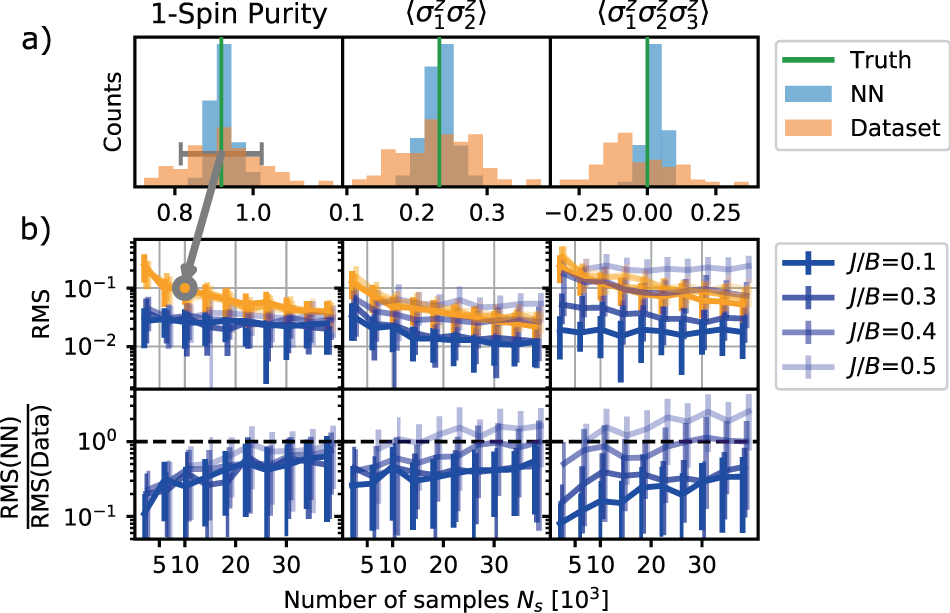
In 2024, Wei and collaborators proposed neural-shadow quantum state tomography using an infidelity-related training objective estimated from classical shadows, including numerical phase-reconstruction comparisons. Other experimental analysis has combined quantum measurement data and machine-learning models to predict many-body observables. These methods differ substantially in objective and guarantee from fitting an RBM solely to one measurement basis; grouping them under the name “AI tomography” should not conceal those differences. [10][12]

Classical shadows and quantum measurement reconstruction in neural experimental data analysis — Experimental quantum data analysis and use of classical shadows to extract information beyond a direct observable average. A separate machine-learning application, not the same method as an RBM wavefunction fit. *Nature Communications* (2024), Fig. 2; CC BY 4.0. Original paper and image credit.

The overlooked problem is identifiability, not just computation

The key limitation is elementary but easy to neglect. A model can fit all collected probabilities perfectly while still being the wrong quantum state. If the measurements never distinguish certain relative phases or nonlocal correlations, an optimizer is free to choose any state consistent with those data. Regularization, physical assumptions and training examples can select a plausible answer, but they do not turn an underdetermined inverse problem into a unique one. [2][4][11]

An instructive two-qubit example uses Bell states with different signs. They generate identical correlated results in the computational basis, but differ for appropriate X-basis measurements. A network trained only on computational-basis counts cannot determine which relative phase was prepared without additional information about the state family or experiment.

|\Phi_{\pm}\rangle=\frac{|00\rangle\pm|11\rangle}{\sqrt2},\qquad p_Z(00)=p_Z(11)=\frac12

The two states have different expectations for X ⊗ X: +1 for Φ₊ and −1 for Φ₋. This supplies a sharp validation test. If a claimed neural reconstruction recovers the sign, either its measurements were sensitive to it or its physical prior selected it. A credible publication must explain which. Reconstructing arbitrary unknown states from insufficient measurements is impossible for reasons of information theory, regardless of network depth.

What can be learned from experimental noise

Neural models have also been used to mitigate state-preparation and measurement errors. For a simple independent bit-flip readout channel, recorded frequencies are a noisy linear transformation of ideal probabilities. If the confusion matrix is calibrated, the likelihood used in training can include that channel, reducing systematic bias without pretending that noisy measurements were perfect. The RBM Rydberg work explicitly modeled certain known experimental errors. [5]

p_{\mathrm{obs}}(y)=\sum_x C_{y|x}\,p_{\theta}(x)

Here C is a calibrated conditional distribution of observed outcome y given ideal outcome x. In a many-qubit experiment it may not factorize into independent single-qubit channels because correlated readout errors can occur. Calibration itself is uncertain, and inverse correction can amplify statistical noise. The 2024 constrained-measurement study by Ma and collaborators explores neural density-matrix estimation under limited copies, incomplete observables and noisy statistics, emphasizing improvements relative to specified baselines rather than universal immunity to errors. [11]

The quantum detector that should be benchmarked

A research-grade tomography comparison should begin with a finite, explicitly defined state family, a measurement budget and a held-out validation task. One baseline reconstructs a density matrix through regularized maximum likelihood. Another fits a pure or mixed neural ansatz using identical measurement settings. A third uses randomized measurements to estimate only the target observables. All methods should receive comparable calibration information, and the analysis should report uncertainty across preparations, random seeds and measurement choices.

Useful stress tests include GHZ-state relative phases, entanglement entropy in short spin chains, states outside the training Hamiltonian family and readout noise with correlations absent from the fit model. A neural model that reproduces training bitstrings but fails on a complementary Pauli basis has learned an incomplete classical shadow of the experiment, not a faithful quantum state. Conversely, agreement on truly withheld noncommuting observables and a well-specified fidelity bound would be persuasive evidence that the model is capturing genuinely quantum structure.

Recent experiments continue to explore this frontier, including 2026 work benchmarking neural ansätze on four-photon entangled systems. Such comparisons expose real differences among positive-amplitude, general pure-state and purification-based mixed-state methods under incomplete measurement data. The promising direction is not to declare one architecture universally superior, but to match the representation and measurement protocol to the experimental state family and the observable accuracy required. [14]

What the detector has really found

The Bloch sphere is a useful metaphor for one qubit. A many-qubit wavefunction has no equally simple spatial portrait, which is precisely why neural state models are interesting. They can compress and interpolate measured quantum correlations when those correlations arise from learnable structure. They can make predictions that would be awkward to obtain from raw bitstrings alone, and they can expose mismatches between hardware behavior and the physical model used to describe it.

But a neural network is not a device for bypassing the uncertainty principle or the limits of measurement. It is a proposed mathematical description of the statistical evidence, together with prior assumptions about what the experiment could have prepared. The most exciting moment is therefore not when the network produces an impressive reconstructed plot. It is when that plot predicts a phase-sensitive measurement, an entanglement property or an error mechanism that was not supplied during fitting and the apparatus confirms the prediction. That is when the wavefunction detective has found something worth trusting.

References

[1] Carleo, G. and Troyer, M. (2017), Solving the Quantum Many-Body Problem with Artificial Neural Networks. https://doi.org/10.1126/science.aag2302.

[2] Torlai, G. et al. (2018), Neural-network quantum state tomography. https://doi.org/10.1038/s41567-018-0048-5.

[3] Torlai, G. and Melko, R. G. (2018), Latent Space Purification via Neural Density Operators. https://doi.org/10.1103/PhysRevLett.120.240503.

[4] Carrasquilla, J. et al. (2019), Reconstructing quantum states with generative models. https://doi.org/10.1038/s42256-019-0028-1.

[5] Torlai, G. et al. (2019), Integrating Neural Networks with a Quantum Simulator for State Reconstruction. https://doi.org/10.1103/PhysRevLett.123.230504.

[6] Xin, T. et al. (2019), Local-measurement-based quantum state tomography via neural networks. https://doi.org/10.1038/s41534-019-0222-3.

[7] Palmieri, A. M. et al. (2020), Experimental neural network enhanced quantum tomography. https://doi.org/10.1038/s41534-020-0248-6.

[8] Schmale, T., Reh, M. and Gärttner, M. (2022), Efficient quantum state tomography with convolutional neural networks. https://doi.org/10.1038/s41534-022-00621-4.

[9] Huang, H.-Y., Kueng, R. and Preskill, J. (2020), Predicting many properties of a quantum system from very few measurements. https://doi.org/10.1038/s41567-020-0932-7.

[10] Wei, V. et al. (2024), Neural-shadow quantum state tomography. https://doi.org/10.1103/PhysRevResearch.6.023250.

[11] Ma, H. et al. (2024), Neural networks for quantum state tomography with constrained measurements. https://doi.org/10.1007/s11128-024-04522-7.

[12] Machine learning on quantum experimental data (2024), Machine learning on quantum experimental data toward solving quantum many-body problems. https://doi.org/10.1038/s41467-024-51932-3.

[13] Haah, J., Harrow, A. W., Ji, Z., Wu, X. and Yu, N. (2017), Sample-optimal tomography of quantum states. https://doi.org/10.1109/TIT.2016.2618030.

[14] Chen, S. et al. (2026), Neural-network quantum state tomography in four-photon entanglement systems. https://doi.org/10.1016/j.optcom.2026.132946.