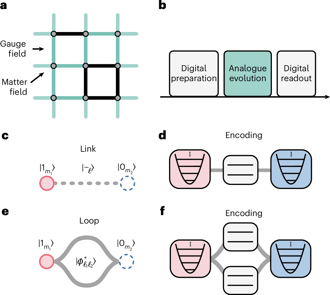
When Magnetic Flux Stops a Particle: A Quantum Loop Built from Trapped Ions

In an ordinary interferometer, magnetic flux changes the phase accumulated by a particle travelling around a loop. In a new trapped-ion experiment, the flux itself belongs to a quantum register. When its value changes from zero to a discrete half-turn, a particle that previously moved between two sites becomes unable to tunnel.

The result, published on 25 September 2026 in Nature Physics by Sebastian Saner and colleagues at Oxford, is an experimental realization of Aharonov–Bohm interference in a small lattice gauge theory with both dynamical matter and dynamical gauge fields. Two vibrational modes encode the matter sites; two electronic qubits encode the gauge links. The experiment is deliberately minimal, but the distinction from an ordinary interference demonstration is substantial. The field is not simply a fixed classical parameter inserted into a particle Hamiltonian. It is an addressable quantum degree of freedom, constrained together with matter by a local gauge symmetry. [1]

That distinction connects a century-old question about electromagnetic potentials to current problems in quantum simulation, topological matter and quantum information. It also provides a useful case study in how the physical hardware of a simulator can encode a field theory without replacing every bosonic excitation by a large collection of qubits.

Why the path around a loop matters

The original Aharonov–Bohm effect concerns a charged particle whose wavefunction can travel around a region containing magnetic flux. Even if the particle moves only where the magnetic field vanishes, the vector potential can change the relative phase of the two paths. The physically measurable quantity is not the potential at a point, which depends on gauge convention, but the phase accumulated around the closed contour. For charge q and enclosed flux Φ, the continuum expression is

\phi_{\mathrm{AB}}=\frac{q}{\hbar}\oint_{\mathcal C}\mathbf A\cdot d\boldsymbol\ell=\frac{q\Phi}{\hbar}\pmod{2\pi}.

Two amplitudes therefore interfere as $A_{\mathrm{tot}}=A_1+A_2e^{i\phi_{\mathrm{AB}}}$ . If the paths have equal amplitude, the intensity is proportional to $1+\cos\phi_{\mathrm{AB}}$ . A phase of zero reinforces transmission; a phase of π cancels it. This is an interference statement, not a force acting locally on the particle. Aharonov and Bohm made the significance of this distinction explicit in 1959. [3]

A lattice gauge theory replaces continuous space with sites and links. The sites carry matter; the links carry variables that determine how matter may hop while respecting a local symmetry. In a discrete $\mathbb Z_2$ gauge theory the link variable has only two possible signs. Its loop flux is likewise binary, so the possible interference phases are zero and π. That makes the phenomenon unusually transparent while retaining the essential relationship between gauge holonomy and a charged particle's motion. [4–6]

What it means for a gauge field to be quantum

A static flux can be represented by choosing a phase in a Hamiltonian before an experiment begins. A dynamical gauge field must instead have its own Hilbert space, observables and time evolution. In the Oxford implementation, each gauge link is a two-level electronic degree of freedom of a trapped strontium ion. Its Pauli operators $\sigma_\ell^x$ and $\sigma_\ell^z$ play different roles: one labels electric-field configurations and the other enters the matter-hopping term.

Each matter site is a quantized vibrational mode with creation and annihilation operators $a_i^\dagger$ and $a_i$ . The occupation $n_i=a_i^\dagger a_i$ counts phonon excitations. The use of an oscillator is more than a convenient storage trick. A bosonic mode naturally contains the states $|0\rangle,|1\rangle,|2\rangle,\ldots$ ; encoding that same ladder in qubits would require an additional mapping and an explicit occupation cutoff. The demonstrated dynamics mainly probe the one-excitation sector, so the availability of the full ladder should not be confused with a demonstration of arbitrarily large boson occupations. [1,2]

For the simplest link, one qubit and two oscillator modes are sufficient. The target Hamiltonian is

H_{\mathrm{link}}=J\left(a_1^\dagger\sigma_\ell^z a_2+a_2^\dagger\sigma_\ell^z a_1\right)+h\sigma_\ell^x.

The coefficient J sets the gauge-mediated hopping strength, while h sets the electric-field energy. A phonon moving between sites changes the state of the gauge link in the electric-field basis. The qubit is therefore not merely controlling a conventional beam splitter; its transformation is part of the gauge-theory dynamics. The original theoretical scheme was developed in 2024 and subsequently implemented experimentally. [1,2]

**Extended Data Figure 1.** Single-link preparation, spin-echo-protected gauge evolution and conditional measurement sequence. Source: Saner et al., *Nature Physics* (2026), CC BY 4.0. Reproduced without modification.

Gauss's law is a constraint on the Hilbert space

Local gauge invariance means that not every formal combination of matter and link states represents the same physical charge sector. For a single link, the relevant generators are products of link electric field and local matter parity. Writing $P_i=(-1)^{n_i}$ , the generators can be chosen as

G_i=\sigma_\ell^x P_i,\qquad P_i=e^{i\pi n_i},\qquad G_i^2=I.

The Hamiltonian is constructed so that $[H_{\mathrm{link}},G_i]=0$ . Consequently, if the initial state satisfies $G_i|\psi_0\rangle=g_i|\psi_0\rangle$ , the ideal evolution remains in that same sector. The eigenvalues $g_i=\pm1$ encode the local constraint, including any chosen background charges. This is the discrete counterpart of Gauss's law: the configuration of electric flux cannot be changed independently of the charge distribution. [1,4]

The conservation law can be checked directly. The parity operator anticommutes with a bosonic creation or annihilation operator at its site, while $\sigma^x$ anticommutes with $\sigma^z$ . A gauge-mediated hop changes both signs. Their product therefore commutes with the hopping Hamiltonian. This simple algebra explains why the simulator must implement a three-part process involving matter at two sites and the gauge link, rather than independent matter tunnelling plus an unrelated spin flip.

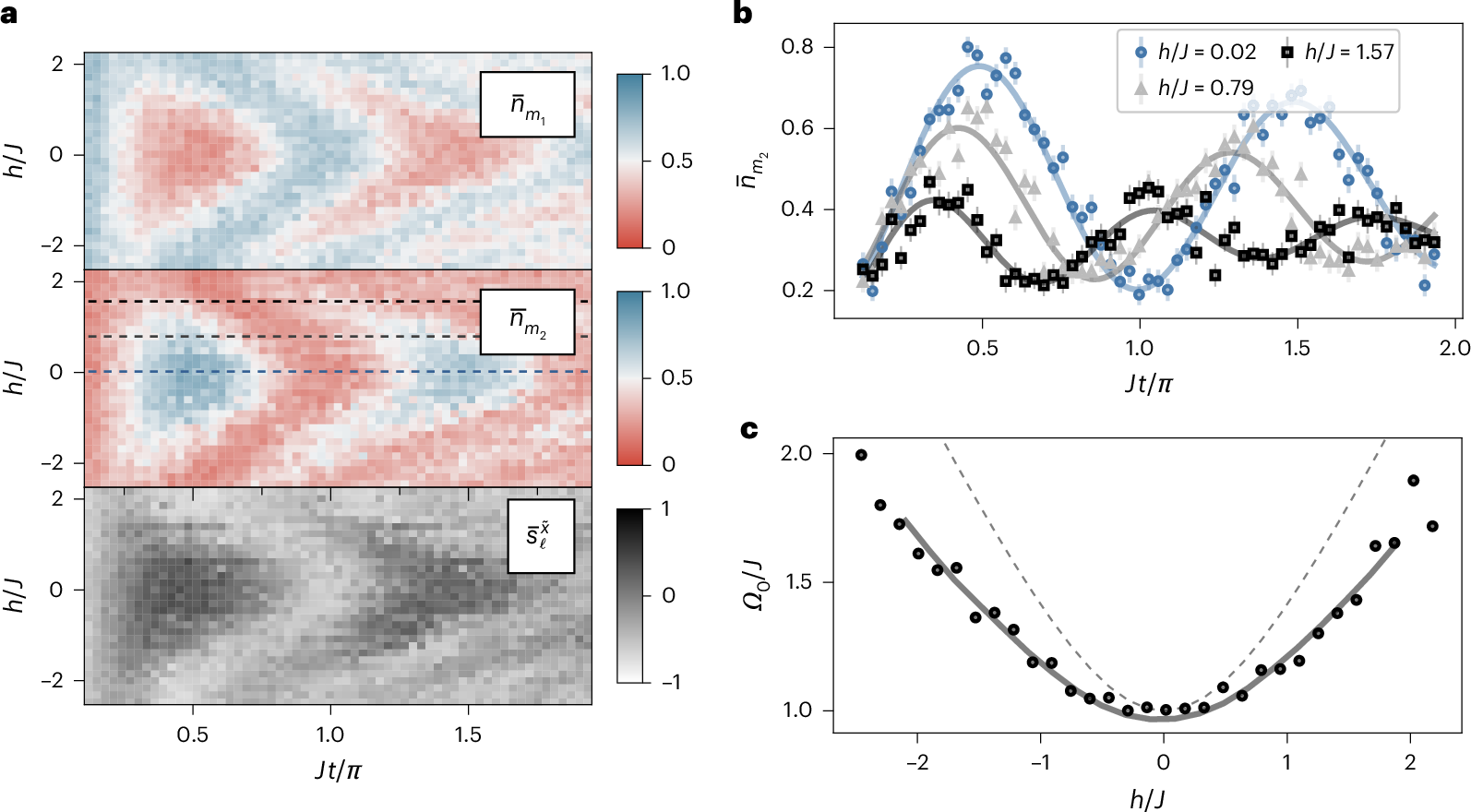
With one initial excitation and vanishing electric energy, the two allowed configurations oscillate coherently. In the ideal two-state sector, the probability of finding the phonon at the second site is

P_2(t)=\sin^2(Jt),\qquad P_1(t)=\cos^2(Jt).

Simultaneously, the link electric-field expectation changes sign. A measurement of matter motion alone would be insufficient to establish the intended gauge dynamics; observing the correlated gauge response supplies the more discriminating test.

**Figure 2.** Measured single-link phonon occupations and link electric field oscillate together as the excitation tunnels; the fit includes a calibrated hopping-rate adjustment. Source: Saner et al., *Nature Physics* (2026), CC BY 4.0. Reproduced without modification.

Electric-field energy changes the tunnelling frequency

When h is nonzero, the two-state Hamiltonian is equivalent, up to a basis convention and an irrelevant overall energy, to $J\sigma^x+h\sigma^z$ . The exact Rabi frequency in this restricted ideal model is $\Omega=\sqrt{J^2+h^2}$ . The matter occupation and the link expectation then follow

\langle n_2(t)\rangle=\frac{J^2}{J^2+h^2}\sin^2\!\left(\sqrt{J^2+h^2}\,t\right),

\langle\sigma_\ell^x(t)\rangle=-1+2\langle n_2(t)\rangle.

The field-energy term has two effects. It increases the oscillation frequency while decreasing the maximum probability that matter reaches the opposite site. These are different observables, and a good experimental comparison should test both rather than equating rapid oscillations with easy transport. In an extended lattice, the cost of rearranging electric strings becomes part of the physics of confinement, although a two-site experiment cannot establish a many-body confining phase by itself. [2,5]

The team measured correlations among the two matter occupations and the gauge-field observable while varying h. Their reported single-link tunnelling rate was approximately $J/\pi=1.47$ kHz in the zero-field experiment; the field-dependent scan gave $J/\pi=1.510(6)$ kHz. The authors also identify a 12% adjustment to the theoretical drive-strength estimate in one comparison. These are calibrated experimental values, not universal constants of the gauge model. [1]

**Figure 3.** Field-dependent matter and gauge dynamics. Increasing the electric energy changes the oscillation frequency and suppresses the transferred population. Source: Saner et al., *Nature Physics* (2026), CC BY 4.0. Reproduced without modification.

Two paths, two links, one magnetic flux

A single link cannot enclose a magnetic flux. To create the smallest loop, the experiment uses two distinct gauge links connecting the same pair of matter sites. Two trapped ions provide the two electronic qubits, while two collective vibrational modes encode the matter. This is a synthetic quasi-two-dimensional geometry: the topology of the encoded graph supplies the loop, not the literal placement of four objects at the corners of a physical square.

The target loop Hamiltonian sums the two gauge-assisted hopping paths:

H_{\mathrm{loop}}=\sum_{\ell=1}^{2}\left[J\left(a_2^\dagger\sigma_\ell^z a_1+a_1^\dagger\sigma_\ell^z a_2\right)+h\sigma_\ell^x\right].

The local generators now contain both links, $G_i=P_i\sigma_1^x\sigma_2^x$ . Their conservation enforces a relation between matter parity and the two electric-field variables. The gauge-invariant magnetic loop operator is $W=\sigma_1^z\sigma_2^z$ , whose eigenvalues are $\pm1$ . In the idealized flux sectors, it supplies the binary holonomy

W=e^{i\phi_{\mathrm{AB}}}\in\{+1,-1\},\qquad\phi_{\mathrm{AB}}\in\{0,\pi\}.

The operator W should not be confused with a local spin measurement. It is a product around the closed path, and its meaning comes from the complete gauge geometry. In this minimal model the loop has two links rather than the four edges of a conventional square plaquette. The distinction matters when extrapolating the result to larger lattice gauge theories. [1,4,5]

Entangled gauge links become the flux register

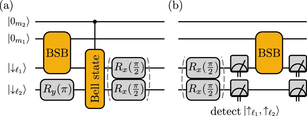
To prepare a definite loop-flux sector, the researchers entangle the two gauge qubits. In the electronic computational basis, the familiar Bell states include

|\Phi^+\rangle=\frac{|\uparrow\uparrow\rangle+|\downarrow\downarrow\rangle}{\sqrt2},\qquad|\Psi^+\rangle=\frac{|\uparrow\downarrow\rangle+|\downarrow\uparrow\rangle}{\sqrt2}.

For the relevant link operator, the first is an eigenstate of $\sigma_1^z\sigma_2^z$ with eigenvalue +1 and the second with eigenvalue −1. They therefore encode the zero- and π-flux sectors. The experiment reports Bell-state preparation fidelity $0.943(9)$ for one of its initial gauge states, a meaningful but imperfect starting point. The relative phase within the Bell superposition also requires calibration because later rotations and correlator measurements are phase sensitive. [1]

For a matter excitation initially localized at site 1, the two path amplitudes add. The simplified effective hopping matrix element is

J_{\mathrm{eff}}=J\left(e^{i\theta_1}+e^{i\theta_2}\right),\qquad |J_{\mathrm{eff}}|^2=4J^2\cos^2\!\left(\frac{\phi_{\mathrm{AB}}}{2}\right).

At zero flux, $|J_{\mathrm{eff}}|=2|J|$ . At π flux, the amplitudes cancel. This formula is an explanatory reduction in a fixed flux sector; the full experiment retains entangled gauge degrees of freedom, which can evolve and become correlated with the moving matter. It is precisely the coexistence of that quantum register with matter dynamics that distinguishes the result from a static-flux analogue.

**Extended Data Figure 3.** Digital preparation and readout sequence for the entangled two-link flux register. Source: Saner et al., *Nature Physics* (2026), CC BY 4.0. Reproduced without modification.

What the measured interference actually shows

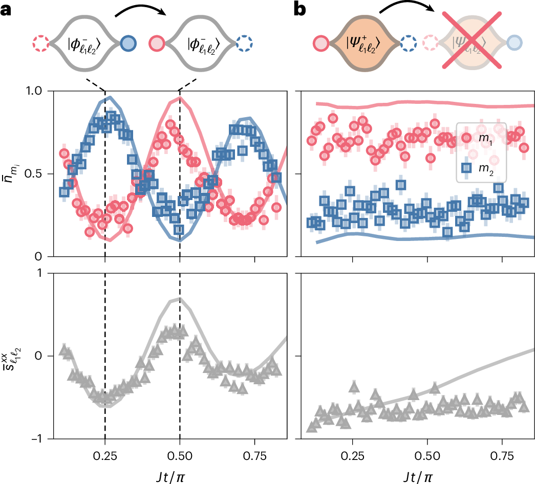
The decisive comparison uses the same two-site matter geometry with different initial Bell states of the links. In the zero-flux configuration, the matter occupation oscillates between sites while a two-link electric correlator changes coherently. The reported loop tunnelling rate is $J/\pi=0.35$ kHz. In the π-flux configuration, the measured matter occupation remains approximately at its initial value and the gauge observables show the corresponding suppression of transport. The observed contrast supports destructive Aharonov–Bohm interference in the encoded $\mathbb Z_2$ theory. [1]

There are two separate claims here. First, the device prepares a gauge-invariant sector with a selected magnetic holonomy. Second, subsequent time evolution exhibits the expected dependence of matter tunnelling on that holonomy. Neither claim requires that an actual charged particle travel around a macroscopic solenoid. The simulated matter consists of phonons and the simulated gauge field consists of electronic qubits. Their controlled Hamiltonian reproduces the targeted mathematical dynamics.

The result is not an observation of a deconfined topological phase in a large two-dimensional material, nor does it demonstrate topologically protected logical qubits. A two-link loop can exhibit flux-sensitive interference without supporting the thermodynamic degeneracy or long-range order associated with topological phases. Its significance is that the fundamental charge–flux interaction is now accessible as a measured dynamical process rather than merely a programmed phase shift.

**Figure 4.** Zero-flux and π-flux loop dynamics. The two initial entangled gauge states produce, respectively, coherent matter tunnelling and inhibited transport. Source: Saner et al., *Nature Physics* (2026), CC BY 4.0. Reproduced without modification.

How a trapped ion implements a gauge-covariant hop

The experimental interaction is engineered using spin-dependent forces on two different motional modes. When the forces couple through noncommuting spin axes, their effective commutator contains a third Pauli operator. In schematic form, $[\sigma^x,\sigma^y]=2i\sigma^z$ . With suitable detunings and pulse shaping, the resulting effective interaction produces the required spin-conditioned exchange of phonon excitations. The design is a concrete example of using a hardware-native interaction to enforce a symmetry instead of repeatedly correcting a generic digital circuit after every elementary operation. [1,2]

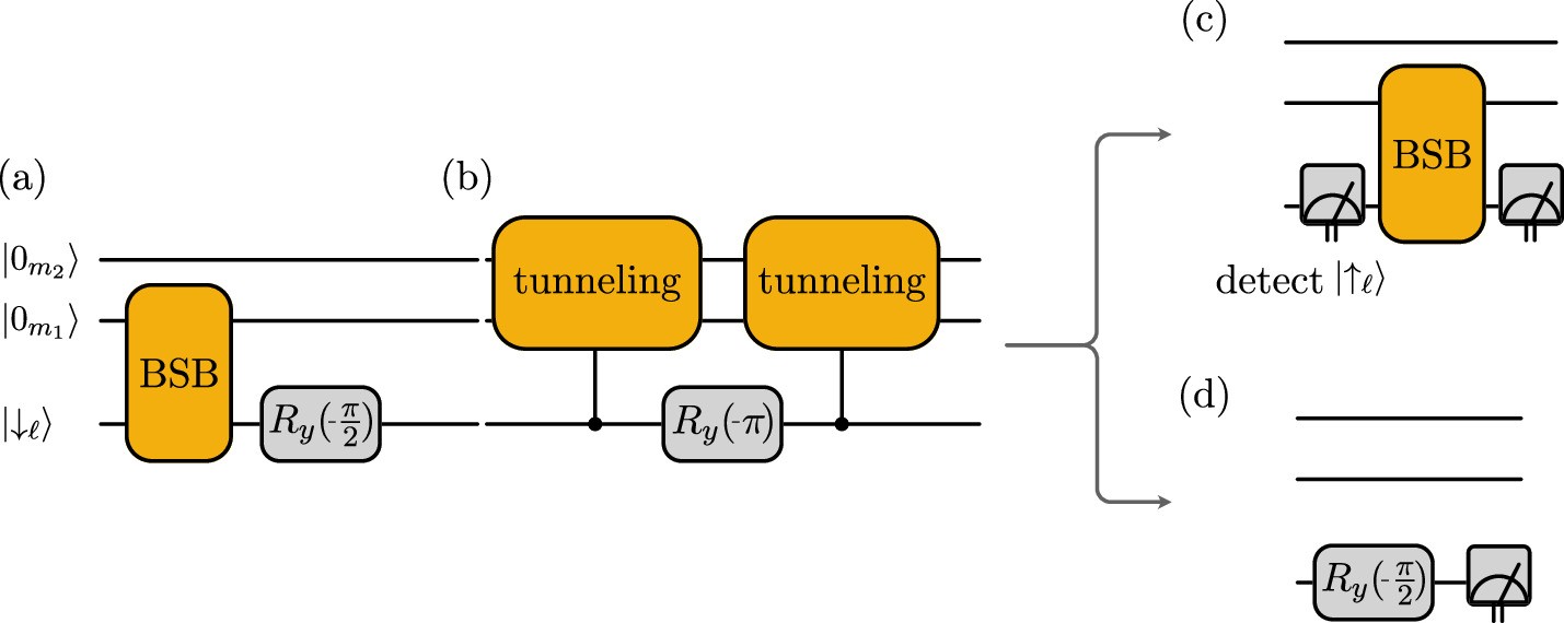
Digital operations still matter. The experiment uses sideband pulses to prepare initial phonon excitations, qubit rotations and entangling operations to prepare the gauge state, echo sequences to suppress unwanted spin dephasing, and state-dependent readout to recover matter and gauge observables. The real-time gauge evolution is then implemented in an analogue interval. Thus the architecture is hybrid in two senses: discrete qubits coexist with bosonic modes, and digital preparation and measurement surround analogue Hamiltonian evolution.

This division of labor avoids a particular resource cost, but it does not eliminate calibration complexity. The normal modes must remain distinguishable; spin-dependent forces require accurate phase and amplitude control; and the measurements used for one oscillator may disturb or delay measurements of the others. A realistic scaling argument must account for these operational demands, not merely count how many abstract qubits were saved.

The leading limitation is a symmetry-breaking physical process

Ideal gauge invariance is an algebraic statement about the designed Hamiltonian. Experimental gauge invariance is a performance question. In the single-link measurements, imperfect cooling and motional heating introduce excitations that need not respect the intended gauge constraint. The paper reports initial thermal occupations around 0.1 for the two modes and heating rates of approximately 300 and 5 quanta per second for the relevant modes in one experiment. These independently measured noise parameters account for much of the reduced oscillation contrast. [1]

A useful diagnostic is the expectation value of the gauge generator. For a state that should remain in a fixed sector, ideal evolution predicts a constant value:

\frac{d}{dt}\langle G_i\rangle=\frac{i}{\hbar}\langle[H,G_i]\rangle=0.

Noise can violate that conservation even when the intended coherent Hamiltonian commutes with the generator. This is why agreement of matter populations with a decaying sinusoid is not enough to certify a gauge simulation. The supplementary analysis compares realistic noisy simulations with a hypothetical case in which oscillator heating is set to zero. The contrast between those curves identifies a concrete experimental target: suppress heating before scaling the geometry. [1]

**Extended Data Figure 4.** Noise simulations contrasting the measured heating environment with an idealized zero-heating case, including the gauge-generator diagnostic. Source: Saner et al., *Nature Physics* (2026), CC BY 4.0. Reproduced without modification.

Why the readout protocol is part of the physics

The researchers measure electronic spin observables using qubit rotations and fluorescence, but the motional modes require mapping their occupations onto an electronic degree of freedom. The single-link protocol includes a conditional readout and postselection, reducing the number of usable shots for some matter observables. This does not invalidate the experiment; it changes the statistical interpretation and should be distinguished from deterministic, single-shot access to every field variable.

Extended Data Figure 1 shows the pulse sequence used to prepare, evolve and read out the minimal link. A spin-echo operation divides the gauge evolution into two intervals while changing the phase convention of the second interaction so that unwanted dephasing is refocused without reversing the desired gauge coupling. Such details determine whether the measured conservation law survives outside an idealized Hamiltonian derivation.

The observable statistics are reported with the associated sampling and postselection conditions. In the single-link scans, the paper used 300 shots for some gauge measurements; matter readout retained a smaller effective sample after conditioning. Such information is essential when interpreting the apparent smoothness of plotted curves and the strength of agreement with a physical noise model.

From a two-link interferometer to larger gauge geometries

The final figure in the paper illustrates how elementary link and loop blocks could be concatenated into larger synthetic lattices, including triangular and tetrahedral building blocks. These are proposed extensions, not devices already demonstrated in the reported work. A larger register would allow flux to move, matter to interact with multiple plaquettes, and electric and magnetic terms to compete over more than one closed path. It could also expose errors that a two-link loop cannot reveal, including crosstalk, correlated heating and imperfect enforcement of many simultaneous Gauss constraints. [1]

The broader motivation is familiar from lattice gauge theory: static equilibrium quantities can sometimes be approached by classical Monte Carlo, whereas real-time dynamics, finite-density regimes and certain sign-problem settings are more difficult. Quantum simulators are attractive because they evolve a physical Hilbert space under an engineered Hamiltonian. Yet no small demonstration should be interpreted as having surpassed the best classical method for its own system size. The present two-site dynamics are readily modeled classically; the experiment tests the control primitives that would be needed for harder cases. [5,6,10,11]

There is also a direct conceptual bridge to quantum error correction. In the toric code, star and plaquette operators constrain physical states, and excitations of different types acquire nontrivial mutual phases when one moves around another. A $\mathbb Z_2$ Wilson loop and the π phase of a vison are closely related mathematical ingredients. Nevertheless, using a gauge simulator to observe interference is not the same as constructing a fault-tolerant memory. The latter additionally requires repeated syndrome extraction, active decoding, logical operations and error-rate scaling. [4,13]

**Figure 5.** Experimentally realized link and loop blocks alongside proposed larger synthetic lattice geometries. The latter are architectural extensions, not demonstrated arrays. Source: Saner et al., *Nature Physics* (2026), CC BY 4.0. Reproduced without modification.

What comes next

The most informative next experiment would preserve both matter and gauge degrees of freedom while increasing the number of independent loops. That would make it possible to distinguish a localized flux defect from a background field, test transport around several paths, and examine how the gauge sector responds when matter is no longer restricted to one excitation. Measurements of Wilson loops, local Gauss generators and matter correlators would need to be collected together, ideally with symmetry-breaking noise independently calibrated.

A companion Nature Physics study published on the same date used a spin–phonon trapped-ion architecture to simulate dynamics of a Yukawa field theory. Its model and objective are different, but the shared design principle is instructive: native oscillator modes can represent bosonic fields without paying the full qubit cost of a Fock-state register. Whether that advantage survives at scale will depend on control fidelity, bosonic heating, measurement overhead and the complexity of coupling many modes. [12]

The Oxford loop experiment makes a narrow but important advance. It turns the sign of a magnetic flux into an experimentally controlled property of entangled gauge qubits and shows how that sign determines whether a matter excitation can travel. The next challenge is not to make the same two-path interference more dramatic. It is to build a lattice large enough that the gauge field develops genuinely many-body behavior while its local constraints remain experimentally trustworthy.

References

S. Saner, O. Băzăvan, D. J. Webb, G. Araneda, C. J. Ballance, R. Srinivas, D. M. Lucas and A. Bermúdez, “Aharonov–Bohm interference in a Z₂ lattice gauge theory on a hybrid qubit–oscillator quantum computer,” Nature Physics 22, 1565–1571 (2026). Source.
O. Băzăvan, S. Saner, E. Tirrito, G. Araneda, R. Srinivas and A. Bermúdez, “Synthetic Z₂ gauge theories based on parametric excitations of trapped ions,” Communications Physics 7, 229 (2024). Source.
Y. Aharonov and D. Bohm, “Significance of Electromagnetic Potentials in the Quantum Theory,” Physical Review 115, 485–491 (1959). Source.
F. J. Wegner, “Duality in Generalized Ising Models and Phase Transitions without Local Order Parameters,” Journal of Mathematical Physics 12, 2259–2272 (1971). Source.
K. G. Wilson, “Confinement of quarks,” Physical Review D 10, 2445–2459 (1974). Source.
J. B. Kogut, “An introduction to lattice gauge theory and spin systems,” Reviews of Modern Physics 51, 659–713 (1979). Source.
E. A. Martinez et al., “Real-time dynamics of lattice gauge theories with a few-qubit quantum computer,” Nature 534, 516–519 (2016). Source.
C. Schweizer et al., “Floquet approach to Z₂ lattice gauge theories with ultracold atoms in optical lattices,” Nature Physics 15, 1168–1173 (2019). Source.
L. Barbiero et al., “Coupling ultracold matter to dynamical gauge fields in optical lattices: From flux attachment to Z₂ lattice gauge theories,” Science Advances 5, eaav7444 (2019). Source.
M. C. Bañuls et al., “Simulating lattice gauge theories within quantum technologies,” European Physical Journal D 74, 165 (2020). Source.
E. Zohar, J. I. Cirac and B. Reznik, “Quantum simulations of lattice gauge theories using ultracold atoms in optical lattices,” Reports on Progress in Physics 79, 014401 (2016). Source.
A. T. Than, S. V. Kadam, V. Vikramaditya et al., “Quantum field theory dynamics on a spin–phonon quantum computer,” Nature Physics (published 25 September 2026). Source.
A. Yu. Kitaev, “Fault-tolerant quantum computation by anyons,” Annals of Physics 303, 2–30 (2003). Source.